Ctrl+K

UXarray Community

  • UXarray Community
  • Catalog
    • UXarray Tutorial and Collaboratory
      • UXarray with CESM-HR on the ne120 Grid
      • Calculus with uxarray
      • Contour Maps of Hurricane Maria on a 15–3 km MPAS Mesh
      • Tropical Cyclones with Neighborhood Filters
    • UXarray’s USCLIVAR Practicum
      • USCLIVAR’s MESACLIP Atmosphere Whole Ensemble Analysis on Native CESM Mesh with UXarray
      • Southern Ocean SST trends: observations vs. CESM-HR vs. CESM-LR / CESM1-LE
  • Repository
  • Open issue
  • .ipynb

Southern Ocean SST trends: observations vs. CESM-HR vs. CESM-LR / CESM1-LE

Contents

  • IMPORTS & DASK CONFIG
  • RUN CONFIG (Native Grid - only for CESM-HR)
  • HELPER FUNCTIONS: LINEAR TREND AND BOX MEAN
  • OBSERVATIONS: ERSSTv5, HadISST1, ERA5
  • CESM-HR: NATIVE GRID (uxarray)
  • CESM-LR: REGRIDDED (aave)
  • CESM1-LE: full ensemble

Southern Ocean SST trends: observations vs. CESM-HR vs. CESM-LR / CESM1-LE#

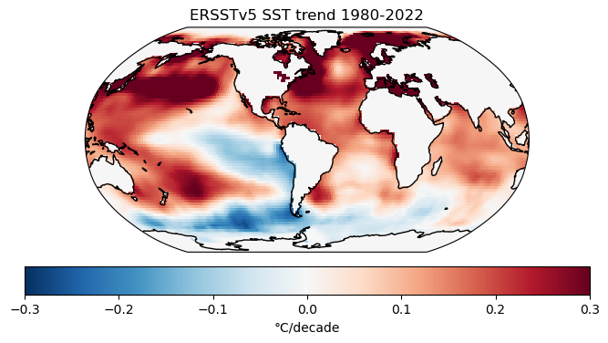
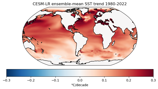
Let us do a linear SST trends comparison between observations, CESM-HR, and CESM-LR similar to that in Figure 1 in the paper entitled Ocean eddy compensation regulates feedbacks amplifying ozone-induced Southern Ocean cooling: linear SST trends (1980-2022) averaged over a South Pacific sector of the Southern Ocean, compared across observational products, CESM-HR (native grid, via uxarray), CESM-LR, and CESM1-LE, plus ensemble-mean spatial trend maps.

Assumptions made explicit here:

  • Trend period: 1980-01 through 2022-12, monthly data, slope reported in °C/decade.

  • CESM-HR: the dedicated native-ocean-grid SST kerchunk product is used directly for members 003-010 — member 002 is excluded because its time coordinate seems corrupted beyond 1929.

IMPORTS & DASK CONFIG#

import re
import gzip
import shutil
from pathlib import Path

import numpy as np
import xarray as xr
import uxarray as ux
import matplotlib.pyplot as plt
import cartopy.crs as ccrs
from dask.distributed import Client

# More headroom per worker than our first PRECT-notebook attempt — fewer, fatter workers.
client = Client(n_workers=10, threads_per_worker=2, memory_limit="7GB")
client.dashboard_link
'/node/crhtc68.hpc.ucar.edu/2846/proxy/8787/status'
import logging
logging.getLogger("distributed.shuffle").setLevel(logging.ERROR)

RUN CONFIG (Native Grid - only for CESM-HR)#

# Determine if notebook is to be run on local device or HPC

# The same pattern as the PRECT notebook) — however, only the CESM-HR kerchunk 
# source has an online-access variant; everything else here (obs products, 
# CESM-LR, CESM1-LE) is only verified to be available on Glade.

RUN_ON = 'hpc'  # 'local' | 'hpc'

if RUN_ON == 'local':
    KERCHUNK_PATH = "https://data.gdex.ucar.edu/d651007/kerchunk/"
    KERCHUNK_ACCESS = "-remote-osdf"
    KERCHUNK_REMOTE_PROTOCOL = "osdf"
    OCN_GRID_FILE = "tx0.1v2_070911.nc"  # would need to be staged locally too
elif RUN_ON == 'hpc':
    KERCHUNK_PATH = "/gdex/data/d651007/kerchunk/"
    KERCHUNK_ACCESS = ""
    KERCHUNK_REMOTE_PROTOCOL = "file"
    OCN_GRID_FILE = "/glade/p/cesmdata/cseg/inputdata/share/scripgrids/tx0.1v2_070911.nc"
# CESM-HR: member 002's dedicated ocean SST kerchunk product has a corrupted time
# axis past 1929; use other members that has clean and complete records.
CESM_HR_MEMBERS = [3, 4, 5, 6, 7, 8, 9, 10]

CESM_LR_PATH = Path("/glade/campaign/univ/utam0017/High-Resolution_Modeling_Workshop_MESACLIP_dataset/CESM_LR/aave")
CESM1LE_SST_PATH = Path("/glade/campaign/cesm/collections/cesmLE/CESM-CAM5-BGC-LE/ocn/proc/tseries/monthly/SST")

ERSSTV5_DIR = Path("/glade/campaign/collections/rda/data/d277009/ersst.v5.nc")
HADISST_GZ = Path("/glade/campaign/collections/rda/data/d277003/HadISST_sst.nc.gz")
ERA5_SST_DIR = Path("/glade/campaign/collections/rda/data/d633001/e5.moda.an.sfc")

# Local cache for the one file that needs decompressing before xarray can open it
CACHE_DIR = Path("./_sst_trend_cache")
CACHE_DIR.mkdir(exist_ok=True)
# Trend period and region
T_START = "1980-01-01"
T_END = "2022-12-31"

BOX_LON = (-180, -60)   # South Pacific sector of the Southern Ocean
BOX_LAT = (-75, -55)    # approximate red-box region from the reference figure

CENTRAL_LON = 300

MONTHS_PER_DECADE = 12 * 10
# Shared colormap/levels for every spatial trend map, matching
# the reference figure's diverging ±0.30 °C/decade scale.
TREND_CMAP = "RdBu_r"
TREND_VMIN, TREND_VMAX = -0.30, 0.30

HELPER FUNCTIONS: LINEAR TREND AND BOX MEAN#

def linear_trend_per_decade(da, time_dim="time"):
    """Can work on both uxarray and xarray data arrays. Ordinary Least Squares (OLS) 
    slope per decade (closed-form cov/var, not a per-point scipy loop) along
    `time_dim`, vectorized over every other dimension. Assumes monthly spacing."""
    n = da.sizes[time_dim]
    t_months = xr.DataArray(np.arange(n, dtype="float64"), dims=time_dim, coords={time_dim: da[time_dim]})
    t_anom = t_months - t_months.mean()
    y_anom = da - da.mean(dim=time_dim, skipna=True)
    slope_per_month = (t_anom * y_anom).sum(dim=time_dim, skipna=True) / (t_anom ** 2).sum(dim=time_dim)
    return slope_per_month * MONTHS_PER_DECADE


def _lon_to_180(lon):
    return ((lon + 180) % 360) - 180


def box_mean_latlon(da, lat_name="lat", lon_name="lon", weights=None):
    """Works only on xarray.DataArray. Area-weighted mean over BOX_LON/BOX_LAT 
    for a regular lat/lon DataArray. Longitude is normalized to -180..180 first 
    (BOX_LON is in that convention) regardless of the source's own convention, 
    then re-sorted since the modulo conversion can break monotonicity."""
    lon = _lon_to_180(da[lon_name])
    da = da.assign_coords({lon_name: lon}).sortby(lon_name)

    lat_vals = da[lat_name].values
    lat_slice = slice(*BOX_LAT) if lat_vals[0] < lat_vals[-1] else slice(*BOX_LAT[::-1])
    da_box = da.sel({lat_name: lat_slice, lon_name: slice(*BOX_LON)})

    if weights is not None:
        w = weights.assign_coords({lon_name: lon}).sortby(lon_name).sel(
            {lat_name: lat_slice, lon_name: slice(*BOX_LON)}
        )
    else:
        # cos(lat) is 1-D; xarray broadcasts it against da_box's other dims
        # (lon, and time if present) automatically in the arithmetic below.
        w = np.cos(np.deg2rad(da_box[lat_name]))
    w = w.where(da_box.notnull())
    return (da_box * w).sum(dim=[lat_name, lon_name], skipna=True) / w.sum(dim=[lat_name, lon_name], skipna=True)


def box_mean_uxarray(uxda):
    """Works only on uxarray.UxDataArray. Area-weighted mean over BOX_LON/BOX_LAT 
    for a UxDataArray, using its own face_areas as weights (zeroed outside the box)."""
    lon = _lon_to_180(uxda.uxgrid.face_lon.values)
    lat = uxda.uxgrid.face_lat.values
    in_box = (lon >= BOX_LON[0]) & (lon <= BOX_LON[1]) & (lat >= BOX_LAT[0]) & (lat <= BOX_LAT[1])
    w = xr.DataArray(np.where(in_box, uxda.uxgrid.face_areas.values, 0.0), dims="n_face")
    return (uxda * w).sum(dim="n_face", skipna=True) / w.sum()

OBSERVATIONS: ERSSTv5, HadISST1, ERA5#

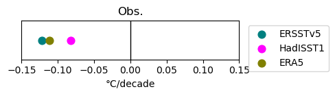
  • ERSSTv5: ersst.v5.nc is a directory of one file per month — sst in °C, 2° grid, longitude 0-360.

  • HadISST1: a single global monthly file, but distributed gzip-compressed (HadISST_sst.nc.gz) — decompressed once into a local cache directory since xarray can’t read a gzip-compressed netCDF container directly. Longitude is already -180..180; missing/land values use a large negative fill value, not NaN, so those get masked explicitly. 1° grid.

  • ERA5: one file per year, variable SSTK in Kelvin — converted to °C, 0.25° grid.

def open_ersstv5(t0=T_START, t1=T_END):
    hits = sorted(ERSSTV5_DIR.glob("ersst.v5.??????.nc"))
    hits = [p for p in hits if t0[:4] + t0[5:7] <= p.name.split(".")[2] <= t1[:4] + t1[5:7]]
    ds = xr.open_mfdataset(hits, combine="nested", concat_dim="time", chunks={"time": 60})
    return ds["sst"].isel(lev=0, drop=True)
%%time
sst_ersstv5 = open_ersstv5()
sst_ersstv5
/glade/work/oero/conda-envs/uxarray-usclivar/lib/python3.14/site-packages/tqdm/auto.py:21: TqdmWarning: IProgress not found. Please update jupyter and ipywidgets. See https://ipywidgets.readthedocs.io/en/stable/user_install.html
  from .autonotebook import tqdm as notebook_tqdm
CPU times: user 5.64 s, sys: 1.07 s, total: 6.72 s
Wall time: 18.8 s
<xarray.DataArray 'sst' (time: 516, lat: 89, lon: 180)> Size: 33MB
dask.array<getitem, shape=(516, 89, 180), dtype=float32, chunksize=(1, 89, 180), chunktype=numpy.ndarray>
Coordinates:
  * time     (time) object 4kB 1980-01-01 00:00:00 ... 2022-12-15
  * lat      (lat) float64 712B -88.0 -86.0 -84.0 -82.0 ... 82.0 84.0 86.0 88.0
  * lon      (lon) float64 1kB 0.0 2.0 4.0 6.0 8.0 ... 352.0 354.0 356.0 358.0
Attributes:
    long_name:      Extended reconstructed sea surface temperature
    standard_name:  sea_surface_temperature
    units:          degree_C
    valid_min:      -3.0
    valid_max:      45.0
xarray.DataArray
'sst'
  • time: 516
  • lat: 89
  • lon: 180
  • dask.array<chunksize=(1, 89, 180), meta=np.ndarray>
    Array Chunk
    Bytes 31.53 MiB 62.58 kiB
    Shape (516, 89, 180) (1, 89, 180)
    Dask graph 516 chunks in 1034 graph layers
    Data type float32 numpy.ndarray
    180 89 516
    • time
      (time)
      object
      1980-01-01 00:00:00 ... 2022-12-15
      long_name :
      Start time of month
      standard_name :
      time
      axis :
      T
      delta_t :
      0000-01-00
      avg_period :
      0000-01-00
      array([cftime.Datetime360Day(1980, 1, 1, 0, 0, 0, 0, has_year_zero=True),
             cftime.Datetime360Day(1980, 2, 1, 0, 0, 0, 0, has_year_zero=True),
             cftime.Datetime360Day(1980, 3, 1, 0, 0, 0, 0, has_year_zero=True), ...,
             Timestamp('2022-10-15 00:00:00'), Timestamp('2022-11-15 00:00:00'),
             Timestamp('2022-12-15 00:00:00')], shape=(516,), dtype=object)
    • lat
      (lat)
      float64
      -88.0 -86.0 -84.0 ... 86.0 88.0
      units :
      degrees_north
      long_name :
      Latitude
      standard_name :
      latitude
      axis :
      Y
      comment :
      Uniform grid from -88 to 88 by 2
      array([-88., -86., -84., -82., -80., -78., -76., -74., -72., -70., -68., -66.,
             -64., -62., -60., -58., -56., -54., -52., -50., -48., -46., -44., -42.,
             -40., -38., -36., -34., -32., -30., -28., -26., -24., -22., -20., -18.,
             -16., -14., -12., -10.,  -8.,  -6.,  -4.,  -2.,   0.,   2.,   4.,   6.,
               8.,  10.,  12.,  14.,  16.,  18.,  20.,  22.,  24.,  26.,  28.,  30.,
              32.,  34.,  36.,  38.,  40.,  42.,  44.,  46.,  48.,  50.,  52.,  54.,
              56.,  58.,  60.,  62.,  64.,  66.,  68.,  70.,  72.,  74.,  76.,  78.,
              80.,  82.,  84.,  86.,  88.])
    • lon
      (lon)
      float64
      0.0 2.0 4.0 ... 354.0 356.0 358.0
      units :
      degrees_east
      long_name :
      Longitude
      standard_name :
      longitude
      axis :
      X
      comment :
      Uniform grid from 0 to 358 by 2
      array([  0.,   2.,   4.,   6.,   8.,  10.,  12.,  14.,  16.,  18.,  20.,  22.,
              24.,  26.,  28.,  30.,  32.,  34.,  36.,  38.,  40.,  42.,  44.,  46.,
              48.,  50.,  52.,  54.,  56.,  58.,  60.,  62.,  64.,  66.,  68.,  70.,
              72.,  74.,  76.,  78.,  80.,  82.,  84.,  86.,  88.,  90.,  92.,  94.,
              96.,  98., 100., 102., 104., 106., 108., 110., 112., 114., 116., 118.,
             120., 122., 124., 126., 128., 130., 132., 134., 136., 138., 140., 142.,
             144., 146., 148., 150., 152., 154., 156., 158., 160., 162., 164., 166.,
             168., 170., 172., 174., 176., 178., 180., 182., 184., 186., 188., 190.,
             192., 194., 196., 198., 200., 202., 204., 206., 208., 210., 212., 214.,
             216., 218., 220., 222., 224., 226., 228., 230., 232., 234., 236., 238.,
             240., 242., 244., 246., 248., 250., 252., 254., 256., 258., 260., 262.,
             264., 266., 268., 270., 272., 274., 276., 278., 280., 282., 284., 286.,
             288., 290., 292., 294., 296., 298., 300., 302., 304., 306., 308., 310.,
             312., 314., 316., 318., 320., 322., 324., 326., 328., 330., 332., 334.,
             336., 338., 340., 342., 344., 346., 348., 350., 352., 354., 356., 358.])
  • long_name :
    Extended reconstructed sea surface temperature
    standard_name :
    sea_surface_temperature
    units :
    degree_C
    valid_min :
    -3.0
    valid_max :
    45.0
%%time
trend_ersstv5 = linear_trend_per_decade(sst_ersstv5).compute()
box_trend_ersstv5 = float(box_mean_latlon(trend_ersstv5))
print("ERSSTv5 box-mean trend (°C/decade):", box_trend_ersstv5)
ERSSTv5 box-mean trend (°C/decade): -0.12173852938450645
CPU times: user 1.39 s, sys: 127 ms, total: 1.52 s
Wall time: 2.78 s
def plot_trend_map_latlon(trend_da, title, lat_name="lat", lon_name="lon", ax=None):
    if ax is None:
        fig, ax = plt.subplots(figsize=(8, 4), subplot_kw={"projection": ccrs.Robinson(central_longitude=CENTRAL_LON)})
    im = ax.pcolormesh(
        trend_da[lon_name], trend_da[lat_name], trend_da,
        transform=ccrs.PlateCarree(), cmap=TREND_CMAP, vmin=TREND_VMIN, vmax=TREND_VMAX,
    )
    ax.coastlines()
    ax.set_title(title)
    return im
%%time
im = plot_trend_map_latlon(trend_ersstv5, "ERSSTv5 SST trend 1980-2022")
plt.colorbar(im, orientation="horizontal", pad=0.05, label="°C/decade")
plt.show()
../../../_images/f0118f88b53908cf5630cdea1dffbc8a8c2cb70988989855077fb9604056edd0.png
CPU times: user 548 ms, sys: 57.7 ms, total: 606 ms
Wall time: 864 ms
def open_hadlsst(t0=T_START, t1=T_END):
    cached = CACHE_DIR / "HadISST_sst.nc"
    if not cached.exists():
        with gzip.open(HADISST_GZ, "rb") as f_in, open(cached, "wb") as f_out:
            shutil.copyfileobj(f_in, f_out)
    ds = xr.open_dataset(cached, chunks={"time": 60})
    sst = ds["sst"].where(ds["sst"] > -900)  # land/missing is a literal -1000.0, not NaN
    return sst.sel(time=slice(t0, t1))


sst_hadisst = open_hadlsst()
sst_hadisst
<xarray.DataArray 'sst' (time: 516, latitude: 180, longitude: 360)> Size: 134MB
dask.array<getitem, shape=(516, 180, 360), dtype=float32, chunksize=(60, 180, 360), chunktype=numpy.ndarray>
Coordinates:
  * time       (time) datetime64[ns] 4kB 1980-01-16T12:00:00 ... 2022-12-16T1...
  * latitude   (latitude) float32 720B 89.5 88.5 87.5 86.5 ... -87.5 -88.5 -89.5
  * longitude  (longitude) float32 1kB -179.5 -178.5 -177.5 ... 178.5 179.5
Attributes:
    standard_name:  sea_surface_temperature
    long_name:      sst
    units:          C
    cell_methods:   time: lat: lon: mean
xarray.DataArray
'sst'
  • time: 516
  • latitude: 180
  • longitude: 360
  • dask.array<chunksize=(60, 180, 360), meta=np.ndarray>
    Array Chunk
    Bytes 127.55 MiB 14.83 MiB
    Shape (516, 180, 360) (60, 180, 360)
    Dask graph 9 chunks in 5 graph layers
    Data type float32 numpy.ndarray
    360 180 516
    • time
      (time)
      datetime64[ns]
      1980-01-16T12:00:00 ... 2022-12-...
      long_name :
      Time
      standard_name :
      time
      array(['1980-01-16T12:00:00.000000000', '1980-02-15T12:00:00.000000000',
             '1980-03-16T12:00:00.000000000', ..., '2022-10-16T12:00:00.000000000',
             '2022-11-16T00:00:00.000000000', '2022-12-16T12:00:00.000000000'],
            shape=(516,), dtype='datetime64[ns]')
    • latitude
      (latitude)
      float32
      89.5 88.5 87.5 ... -88.5 -89.5
      units :
      degrees_north
      long_name :
      Latitude
      standard_name :
      latitude
      array([ 89.5,  88.5,  87.5,  86.5,  85.5,  84.5,  83.5,  82.5,  81.5,  80.5,
              79.5,  78.5,  77.5,  76.5,  75.5,  74.5,  73.5,  72.5,  71.5,  70.5,
              69.5,  68.5,  67.5,  66.5,  65.5,  64.5,  63.5,  62.5,  61.5,  60.5,
              59.5,  58.5,  57.5,  56.5,  55.5,  54.5,  53.5,  52.5,  51.5,  50.5,
              49.5,  48.5,  47.5,  46.5,  45.5,  44.5,  43.5,  42.5,  41.5,  40.5,
              39.5,  38.5,  37.5,  36.5,  35.5,  34.5,  33.5,  32.5,  31.5,  30.5,
              29.5,  28.5,  27.5,  26.5,  25.5,  24.5,  23.5,  22.5,  21.5,  20.5,
              19.5,  18.5,  17.5,  16.5,  15.5,  14.5,  13.5,  12.5,  11.5,  10.5,
               9.5,   8.5,   7.5,   6.5,   5.5,   4.5,   3.5,   2.5,   1.5,   0.5,
              -0.5,  -1.5,  -2.5,  -3.5,  -4.5,  -5.5,  -6.5,  -7.5,  -8.5,  -9.5,
             -10.5, -11.5, -12.5, -13.5, -14.5, -15.5, -16.5, -17.5, -18.5, -19.5,
             -20.5, -21.5, -22.5, -23.5, -24.5, -25.5, -26.5, -27.5, -28.5, -29.5,
             -30.5, -31.5, -32.5, -33.5, -34.5, -35.5, -36.5, -37.5, -38.5, -39.5,
             -40.5, -41.5, -42.5, -43.5, -44.5, -45.5, -46.5, -47.5, -48.5, -49.5,
             -50.5, -51.5, -52.5, -53.5, -54.5, -55.5, -56.5, -57.5, -58.5, -59.5,
             -60.5, -61.5, -62.5, -63.5, -64.5, -65.5, -66.5, -67.5, -68.5, -69.5,
             -70.5, -71.5, -72.5, -73.5, -74.5, -75.5, -76.5, -77.5, -78.5, -79.5,
             -80.5, -81.5, -82.5, -83.5, -84.5, -85.5, -86.5, -87.5, -88.5, -89.5],
            dtype=float32)
    • longitude
      (longitude)
      float32
      -179.5 -178.5 ... 178.5 179.5
      units :
      degrees_east
      long_name :
      Longitude
      standard_name :
      longitude
      array([-179.5, -178.5, -177.5, ...,  177.5,  178.5,  179.5],
            shape=(360,), dtype=float32)
  • standard_name :
    sea_surface_temperature
    long_name :
    sst
    units :
    C
    cell_methods :
    time: lat: lon: mean
%%time
box_series_hadisst = box_mean_latlon(sst_hadisst, lat_name="latitude", lon_name="longitude")
box_trend_hadisst = float(linear_trend_per_decade(box_series_hadisst).compute())
print("HadISST1 box-mean trend (°C/decade):", box_trend_hadisst)
HadISST1 box-mean trend (°C/decade): -0.08234362182302288
CPU times: user 106 ms, sys: 15 ms, total: 121 ms
Wall time: 203 ms
def open_era5_sst(t0=T_START, t1=T_END):
    years = range(int(t0[:4]), int(t1[:4]) + 1)
    hits = []
    for y in years:
        hits += sorted((ERA5_SST_DIR / str(y)).glob(f"e5.moda.an.sfc.128_034_sstk.ll025sc.{y}*.nc"))
    ds = xr.open_mfdataset(hits, combine="by_coords", chunks={"time": 12})
    sstk = ds["SSTK"].sel(time=slice(t0, t1))
    sst = sstk - 273.15
    sst.attrs["units"] = "degC"
    return sst
%%time
sst_era5 = open_era5_sst()
sst_era5
CPU times: user 486 ms, sys: 191 ms, total: 677 ms
Wall time: 2.41 s
<xarray.DataArray 'SSTK' (time: 516, latitude: 721, longitude: 1440)> Size: 2GB
dask.array<sub, shape=(516, 721, 1440), dtype=float32, chunksize=(12, 389, 776), chunktype=numpy.ndarray>
Coordinates:
  * time       (time) datetime64[ns] 4kB 1980-01-01 1980-02-01 ... 2022-12-01
  * latitude   (latitude) float64 6kB 90.0 89.75 89.5 ... -89.5 -89.75 -90.0
  * longitude  (longitude) float64 12kB 0.0 0.25 0.5 0.75 ... 359.2 359.5 359.8
Attributes: (12/14)
    long_name:                     Sea surface temperature
    short_name:                    sstk
    units:                         degC
    original_format:               WMO GRIB 1 with ECMWF local table
    ecmwf_local_table:             128
    ecmwf_parameter:               34
    ...                            ...
    grid_specification:            0.25 degree x 0.25 degree from 90N to 90S ...
    rda_dataset:                   ds633.1
    rda_dataset_url:               https:/rda.ucar.edu/datasets/ds633.1/
    rda_dataset_doi:               DOI: 10.5065/P8GT-0R61
    rda_dataset_group:             ERA5 monthly mean atmospheric surface anal...
    number_of_significant_digits:  7
xarray.DataArray
'SSTK'
  • time: 516
  • latitude: 721
  • longitude: 1440
  • dask.array<chunksize=(12, 389, 776), meta=np.ndarray>
    Array Chunk
    Bytes 2.00 GiB 13.82 MiB
    Shape (516, 721, 1440) (12, 389, 776)
    Dask graph 172 chunks in 88 graph layers
    Data type float32 numpy.ndarray
    1440 721 516
    • time
      (time)
      datetime64[ns]
      1980-01-01 ... 2022-12-01
      long_name :
      time
      array(['1980-01-01T00:00:00.000000000', '1980-02-01T00:00:00.000000000',
             '1980-03-01T00:00:00.000000000', ..., '2022-10-01T00:00:00.000000000',
             '2022-11-01T00:00:00.000000000', '2022-12-01T00:00:00.000000000'],
            shape=(516,), dtype='datetime64[ns]')
    • latitude
      (latitude)
      float64
      90.0 89.75 89.5 ... -89.75 -90.0
      long_name :
      latitude
      short_name :
      lat
      units :
      degrees_north
      array([ 90.  ,  89.75,  89.5 , ..., -89.5 , -89.75, -90.  ], shape=(721,))
    • longitude
      (longitude)
      float64
      0.0 0.25 0.5 ... 359.2 359.5 359.8
      long_name :
      longitude
      short_name :
      lon
      units :
      degrees_east
      array([0.0000e+00, 2.5000e-01, 5.0000e-01, ..., 3.5925e+02, 3.5950e+02,
             3.5975e+02], shape=(1440,))
  • long_name :
    Sea surface temperature
    short_name :
    sstk
    units :
    degC
    original_format :
    WMO GRIB 1 with ECMWF local table
    ecmwf_local_table :
    128
    ecmwf_parameter :
    34
    minimum_value :
    269.61328
    maximum_value :
    307.48218
    grid_specification :
    0.25 degree x 0.25 degree from 90N to 90S and 0E to 359.75E (721 x 1440 Latitude/Longitude)
    rda_dataset :
    ds633.1
    rda_dataset_url :
    https:/rda.ucar.edu/datasets/ds633.1/
    rda_dataset_doi :
    DOI: 10.5065/P8GT-0R61
    rda_dataset_group :
    ERA5 monthly mean atmospheric surface analysis [netCDF4]
    number_of_significant_digits :
    7
%%time
box_series_era5 = box_mean_latlon(sst_era5, lat_name="latitude", lon_name="longitude")
box_trend_era5 = float(linear_trend_per_decade(box_series_era5).compute())
print("ERA5 box-mean trend (°C/decade):", box_trend_era5)
ERA5 box-mean trend (°C/decade): -0.11181791793345235
CPU times: user 429 ms, sys: 42.6 ms, total: 471 ms
Wall time: 1.54 s
fig, ax = plt.subplots(figsize=(5, 1.5))
obs_trends = {"ERSSTv5": box_trend_ersstv5, "HadISST1": box_trend_hadisst, "ERA5": box_trend_era5}
colors = {"ERSSTv5": "teal", "HadISST1": "magenta", "ERA5": "olive"}
for name, val in obs_trends.items():
    ax.scatter(val, 0, color=colors[name], label=name, s=60, zorder=3)
ax.axvline(0, color="black", lw=1)
ax.set_xlim(-0.15, 0.15)
ax.set_yticks([])
ax.set_xlabel("°C/decade")
ax.legend(loc="upper left", bbox_to_anchor=(1.02, 1.0))
ax.set_title("Obs.")
plt.tight_layout()
plt.show()
../../../_images/4a92ef03c85ddb87c049a0be6caa9c4bd55ac404b7ae5038defae578a88c636d.png

CESM-HR: NATIVE GRID (uxarray)#

The native ocean grid is a ~0.1° curvilinear grid (~8.64M cells) — a SCRIP grid file for it (tx0.1v2_070911.nc) is present in CESM’s shared inputdata dir.

The kerchunk source stores SST as (time, nlat, nlon) though, i.e. not already flattened to one spatial dimension, i.e. n_face in this case; hence, we .stack() into a single n_face dimension before wrapping as a UxDataArray.

This is the most expensive section in the notebook — the global ensemble-mean trend map (like panel F in the reference figure) means computing a per-gridcell linear regression over 516 months × 8 members × 8.64M cells.

%%time
uxgrid_hr_ocn = ux.open_grid(OCN_GRID_FILE)
uxgrid_hr_ocn
CPU times: user 8 s, sys: 1.13 s, total: 9.13 s
Wall time: 3.6 s
<uxarray.Grid>
Original Grid Type: Scrip
Grid Dimensions:
  * n_node: 8644402
  * n_face: 8640000
  * n_max_face_nodes: 4
Grid Coordinates (Spherical):
  * node_lon: (8644402,)
  * node_lat: (8644402,)
  * face_lon: (8640000,)
  * face_lat: (8640000,)
Grid Coordinates (Cartesian):
Grid Connectivity Variables:
  * face_node_connectivity: (8640000, 4)
Grid Descriptor Variables:
uxarray.Grid
    • n_node: 8644402
    • n_face: 8640000
    • n_max_face_nodes: 4
    • node_lon
      (n_node)
      float64
      63.32 -50.97 -99.7 ... 90.55 20.7
      standard_name :
      longitude
      long name :
      Longitude of the corner nodes of each face
      units :
      degrees_east
      array([  63.32210941,  -50.97211845,  -99.7       , ..., -110.17704226,
               90.54503029,   20.7       ], shape=(8644402,))
    • node_lat
      (n_node)
      float64
      68.91 44.34 -46.82 ... 64.52 -3.198
      standard_name :
      latitude
      long name :
      Latitude of the corner nodes of each face
      units :
      degrees_north
      array([ 68.90702174,  44.33676325, -46.82266234, ...,  48.48148498,
              64.51981302,  -3.19841469], shape=(8644402,))
    • face_lon
      (n_face)
      float64
      -109.9 -109.8 ... -110.0 -110.0
      standard_name :
      longitude
      long name :
      Longitude of the center of each face
      units :
      degrees_east
      array([-109.95      , -109.85      , -109.75      , ..., -110.00025596,
             -110.00015531, -110.00005467], shape=(8640000,))
    • face_lat
      (n_face)
      float64
      -84.23 -84.23 ... 62.34 62.34
      standard_name :
      latitude
      long name :
      Latitude of the center of each face
      units :
      degrees_north
      array([-84.22586292, -84.22586292, -84.22586292, ...,  62.33762944,
              62.33740034,  62.33728584], shape=(8640000,))
      • face_node_connectivity
        (n_face, n_max_face_nodes)
        int64
        6629834 7372008 ... 386566 6069344
        cf_role :
        face_node_connectivity
        long name :
        Maps every face to its corner nodes.
        start_index :
        0
        _FillValue :
        -9223372036854775808
        array([[6629834, 7372008, 5543253, 7662877],
               [7372008, 3664925, 2319002, 5543253],
               [3664925, 1241974, 8212026, 2319002],
               ...,
               [5914778, 2933489, 2002633, 8404807],
               [2933489, 6969606, 6069344, 2002633],
               [6969606, 4159269,  386566, 6069344]], shape=(8640000, 4))
      • source_grid_spec :
        Scrip
      def open_hr_sst_member(member, t0=T_START, t1=T_END):
          hits = sorted(Path(KERCHUNK_PATH).glob(f"*.{member:03d}.ocn.month_1.sst_only{KERCHUNK_ACCESS}.parq"))
          if not hits:
              return None
      
          ds = xr.open_dataset(
              str(hits[0]), engine="kerchunk", decode_timedelta=False,
              decode_times=xr.coders.CFDatetimeCoder(use_cftime=True),
              chunks={"time": 60},
              
              # To avoid the "boolean value of NA is ambiguous" error.
              storage_options={"remote_protocol": KERCHUNK_REMOTE_PROTOCOL},
          )
          sst = ds["SST"].sel(time=slice(t0, t1))
          
          # Flatten (nlat, nlon) -> n_face
          sst = sst.stack(n_face=("nlat", "nlon")).reset_index("n_face", drop=True)
          
          return ux.UxDataArray(sst, uxgrid=uxgrid_hr_ocn)
      
      %%time
      # Opened lazily only (similar to the first notebook, i.e. PRECT)
      hr_members = {m: open_hr_sst_member(m) for m in CESM_HR_MEMBERS}
      hr_members[CESM_HR_MEMBERS[0]]
      
      CPU times: user 2.01 s, sys: 352 ms, total: 2.36 s
      Wall time: 3.37 s
      
      <xarray.UxDataArray 'SST' (time: 313, n_face: 8640000)> Size: 11GB
      dask.array<reshape, shape=(313, 8640000), dtype=float32, chunksize=(60, 104400), chunktype=numpy.ndarray>
      Coordinates:
        * time     (time) object 3kB 1980-01-01 00:00:00 ... 2006-01-01 00:00:00
          TLAT     (time, n_face) float64 22GB dask.array<chunksize=(1, 345600), meta=np.ndarray>
          TLONG    (time, n_face) float64 22GB dask.array<chunksize=(1, 345600), meta=np.ndarray>
          ULAT     (time, n_face) float64 22GB dask.array<chunksize=(1, 345600), meta=np.ndarray>
          ULONG    (time, n_face) float64 22GB dask.array<chunksize=(1, 345600), meta=np.ndarray>
      Dimensions without coordinates: n_face
      Attributes:
          long_name:     Potential Temperature
          units:         degC
          grid_loc:      3111
          cell_methods:  time: mean z_t: mean
      <xarray.UxDataArray 'SST' (time: 313, n_face: 8640000)> Size: 11GB
      dask.array<reshape, shape=(313, 8640000), dtype=float32, chunksize=(60, 104400), chunktype=numpy.ndarray>
      Coordinates:
        * time     (time) object 3kB 1980-01-01 00:00:00 ... 2006-01-01 00:00:00
          TLAT     (time, n_face) float64 22GB dask.array<chunksize=(1, 345600), meta=np.ndarray>
          TLONG    (time, n_face) float64 22GB dask.array<chunksize=(1, 345600), meta=np.ndarray>
          ULAT     (time, n_face) float64 22GB dask.array<chunksize=(1, 345600), meta=np.ndarray>
          ULONG    (time, n_face) float64 22GB dask.array<chunksize=(1, 345600), meta=np.ndarray>
      Dimensions without coordinates: n_face
      Attributes:
          long_name:     Potential Temperature
          units:         degC
          grid_loc:      3111
          cell_methods:  time: mean z_t: mean
      uxarray.UxDataArray
      'SST'
      • time: 313
      • n_face: 8640000
      • dask.array<chunksize=(1, 104400), meta=np.ndarray>
        Array Chunk
        Bytes 10.07 GiB 23.90 MiB
        Shape (313, 8640000) (60, 104400)
        Dask graph 630 chunks in 6 graph layers
        Data type float32 numpy.ndarray
        8640000 313
        • time
          (time)
          object
          1980-01-01 00:00:00 ... 2006-01-...
          long_name :
          time
          bounds :
          time_bound
          array([cftime.DatetimeNoLeap(1980, 1, 1, 0, 0, 0, 0, has_year_zero=True),
                 cftime.DatetimeNoLeap(1980, 2, 1, 0, 0, 0, 0, has_year_zero=True),
                 cftime.DatetimeNoLeap(1980, 3, 1, 0, 0, 0, 0, has_year_zero=True), ...,
                 cftime.DatetimeNoLeap(2005, 11, 1, 0, 0, 0, 0, has_year_zero=True),
                 cftime.DatetimeNoLeap(2005, 12, 1, 0, 0, 0, 0, has_year_zero=True),
                 cftime.DatetimeNoLeap(2006, 1, 1, 0, 0, 0, 0, has_year_zero=True)],
                shape=(313,), dtype=object)
        • TLAT
          (time, n_face)
          float64
          dask.array<chunksize=(1, 345600), meta=np.ndarray>
          long_name :
          array of t-grid latitudes
          units :
          degrees_north
          Array Chunk
          Bytes 20.15 GiB 158.20 MiB
          Shape (313, 8640000) (60, 345600)
          Dask graph 175 chunks in 5 graph layers
          Data type float64 numpy.ndarray
          8640000 313
        • TLONG
          (time, n_face)
          float64
          dask.array<chunksize=(1, 345600), meta=np.ndarray>
          long_name :
          array of t-grid longitudes
          units :
          degrees_east
          Array Chunk
          Bytes 20.15 GiB 158.20 MiB
          Shape (313, 8640000) (60, 345600)
          Dask graph 175 chunks in 5 graph layers
          Data type float64 numpy.ndarray
          8640000 313
        • ULAT
          (time, n_face)
          float64
          dask.array<chunksize=(1, 345600), meta=np.ndarray>
          long_name :
          array of u-grid latitudes
          units :
          degrees_north
          Array Chunk
          Bytes 20.15 GiB 158.20 MiB
          Shape (313, 8640000) (60, 345600)
          Dask graph 175 chunks in 5 graph layers
          Data type float64 numpy.ndarray
          8640000 313
        • ULONG
          (time, n_face)
          float64
          dask.array<chunksize=(1, 345600), meta=np.ndarray>
          long_name :
          array of u-grid longitudes
          units :
          degrees_east
          Array Chunk
          Bytes 20.15 GiB 158.20 MiB
          Shape (313, 8640000) (60, 345600)
          Dask graph 175 chunks in 5 graph layers
          Data type float64 numpy.ndarray
          8640000 313
        • time
          PandasIndex
          PandasIndex(CFTimeIndex([1980-01-01 00:00:00, 1980-02-01 00:00:00, 1980-03-01 00:00:00,
                       1980-04-01 00:00:00, 1980-05-01 00:00:00, 1980-06-01 00:00:00,
                       1980-07-01 00:00:00, 1980-08-01 00:00:00, 1980-09-01 00:00:00,
                       1980-10-01 00:00:00,
                       ...
                       2005-04-01 00:00:00, 2005-05-01 00:00:00, 2005-06-01 00:00:00,
                       2005-07-01 00:00:00, 2005-08-01 00:00:00, 2005-09-01 00:00:00,
                       2005-10-01 00:00:00, 2005-11-01 00:00:00, 2005-12-01 00:00:00,
                       2006-01-01 00:00:00],
                      dtype='object', length=313, calendar='noleap', freq='MS'))
      • long_name :
        Potential Temperature
        units :
        degC
        grid_loc :
        3111
        cell_methods :
        time: mean z_t: mean
      Show Grid Information
      <uxarray.Grid>
      Original Grid Type: Scrip
      Grid Dimensions:
        * n_node: 8644402
        * n_face: 8640000
        * n_max_face_nodes: 4
      Grid Coordinates (Spherical):
        * node_lon: (8644402,)
        * node_lat: (8644402,)
        * face_lon: (8640000,)
        * face_lat: (8640000,)
      Grid Coordinates (Cartesian):
      Grid Connectivity Variables:
        * face_node_connectivity: (8640000, 4)
      Grid Descriptor Variables:
      
      uxarray.UxDataArray.uxgrid
        • n_node: 8644402
        • n_face: 8640000
        • n_max_face_nodes: 4
        • node_lon
          (n_node)
          float64
          63.32 -50.97 -99.7 ... 90.55 20.7
          standard_name :
          longitude
          long name :
          Longitude of the corner nodes of each face
          units :
          degrees_east
          array([  63.32210941,  -50.97211845,  -99.7       , ..., -110.17704226,
                   90.54503029,   20.7       ], shape=(8644402,))
        • node_lat
          (n_node)
          float64
          68.91 44.34 -46.82 ... 64.52 -3.198
          standard_name :
          latitude
          long name :
          Latitude of the corner nodes of each face
          units :
          degrees_north
          array([ 68.90702174,  44.33676325, -46.82266234, ...,  48.48148498,
                  64.51981302,  -3.19841469], shape=(8644402,))
        • face_lon
          (n_face)
          float64
          -109.9 -109.8 ... -110.0 -110.0
          standard_name :
          longitude
          long name :
          Longitude of the center of each face
          units :
          degrees_east
          array([-109.95      , -109.85      , -109.75      , ..., -110.00025596,
                 -110.00015531, -110.00005467], shape=(8640000,))
        • face_lat
          (n_face)
          float64
          -84.23 -84.23 ... 62.34 62.34
          standard_name :
          latitude
          long name :
          Latitude of the center of each face
          units :
          degrees_north
          array([-84.22586292, -84.22586292, -84.22586292, ...,  62.33762944,
                  62.33740034,  62.33728584], shape=(8640000,))
          • face_node_connectivity
            (n_face, n_max_face_nodes)
            int64
            6629834 7372008 ... 386566 6069344
            cf_role :
            face_node_connectivity
            long name :
            Maps every face to its corner nodes.
            start_index :
            0
            _FillValue :
            -9223372036854775808
            array([[6629834, 7372008, 5543253, 7662877],
                   [7372008, 3664925, 2319002, 5543253],
                   [3664925, 1241974, 8212026, 2319002],
                   ...,
                   [5914778, 2933489, 2002633, 8404807],
                   [2933489, 6969606, 6069344, 2002633],
                   [6969606, 4159269,  386566, 6069344]], shape=(8640000, 4))
          • source_grid_spec :
            Scrip
          %%time
          # Box-mean trend per member. Cheap (a single area-weighted scalar
          # reduction per member) — build all 8 members' graphs and compute once so dask
          # schedules them as one parallel graph, same pattern as the PRECT ensemble cell.
          hr_box_series = {m: box_mean_uxarray(hr_members[m]) for m in CESM_HR_MEMBERS}
          hr_box_trend_da = xr.concat(
              [linear_trend_per_decade(s) for s in hr_box_series.values()], dim="member"
          ).assign_coords(member=list(hr_box_series.keys()))
          hr_box_trend_da = hr_box_trend_da.compute()
          
          hr_box_trends = dict(zip(hr_box_trend_da["member"].values, hr_box_trend_da.values))
          hr_box_trends
          
          /glade/work/oero/conda-envs/uxarray-usclivar/lib/python3.14/site-packages/distributed/client.py:3429: UserWarning: Sending large graph of size 67.00 MiB.
          This may cause some slowdown.
          Consider loading the data with Dask directly
           or using futures or delayed objects to embed the data into the graph without repetition.
          See also https://docs.dask.org/en/stable/best-practices.html#load-data-with-dask for more information.
            warnings.warn(
          
          CPU times: user 6min 28s, sys: 27.9 s, total: 6min 56s
          Wall time: 11min 37s
          
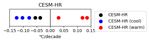
          {np.int64(3): np.float64(0.11841979114758591),
           np.int64(4): np.float64(0.13553071643161477),
           np.int64(5): np.float64(-0.07788712420627877),
           np.int64(6): np.float64(-0.03788274811895097),
           np.int64(7): np.float64(0.030884520900788137),
           np.int64(8): np.float64(-0.1027328436380362),
           np.int64(9): np.float64(-0.1247292156683743),
           np.int64(10): np.float64(-0.05596738388470638)}
          
          # Classify into coolest-3 / warmest-3 / remaining, same idea as the reference
          # figure's panel E (which does this over 10 members; we have 8, so 3 cool + 3
          # warm leaves 2 in the middle instead of 4).
          ranked = sorted(hr_box_trends.items(), key=lambda kv: kv[1])
          cool_members = dict(ranked[:3])
          warm_members = dict(ranked[-3:])
          mid_members = dict(ranked[3:-3])
          
          fig, ax = plt.subplots(figsize=(5, 1.5))
          for members, color, label in [(mid_members, "black", "CESM-HR"),
                                          (cool_members, "blue", "CESM-HR (cool)"),
                                          (warm_members, "red", "CESM-HR (warm)")]:
              ax.scatter(list(members.values()), [0] * len(members), color=color, label=label, s=60, zorder=3)
          ax.axvline(0, color="black", lw=1)
          ax.set_xlim(-0.15, 0.15)
          ax.set_yticks([])
          ax.set_xlabel("°C/decade")
          ax.legend(loc="upper left", bbox_to_anchor=(1.02, 1.0))
          ax.set_title("CESM-HR")
          plt.tight_layout()
          plt.show()
          
          ../../../_images/86c7a5937f4201e6f267e0a71f216d79562d4341ba792126faec02a999ddd499.png
          %%time
          # Ensemble-mean spatial trend map — the expensive one (see markdown
          # above). Mean-of-trends (each member's own trend map, then averaged), not
          # trend-of-the-ensemble-mean-SST — matches how the reference figure's caption
          # phrases "ensemble-mean linear trends in CESM-HR".
          hr_member_trend_maps = [linear_trend_per_decade(hr_members[m]) for m in CESM_HR_MEMBERS]
          hr_ensemble_mean_trend = xr.concat(hr_member_trend_maps, dim="member").mean(dim="member")
          hr_ensemble_mean_trend = hr_ensemble_mean_trend.compute()
          
          CPU times: user 7min 1s, sys: 33.5 s, total: 7min 35s
          Wall time: 14min 50s
          
          hr_ensemble_mean_trend = ux.UxDataArray(hr_ensemble_mean_trend, uxgrid=uxgrid_hr_ocn)
          
          hr_ensemble_mean_trend
          
          <xarray.UxDataArray (n_face: 8640000)> Size: 69MB
          array([0., 0., 0., ..., 0., 0., 0.], shape=(8640000,))
          Dimensions without coordinates: n_face
          Attributes:
              long_name:     Potential Temperature
              units:         degC
              grid_loc:      3111
              cell_methods:  time: mean z_t: mean
          <xarray.UxDataArray (n_face: 8640000)> Size: 69MB
          array([0., 0., 0., ..., 0., 0., 0.], shape=(8640000,))
          Dimensions without coordinates: n_face
          Attributes:
              long_name:     Potential Temperature
              units:         degC
              grid_loc:      3111
              cell_methods:  time: mean z_t: mean
          uxarray.UxDataArray
          • n_face: 8640000
          • 0.0 0.0 0.0 0.0 0.0 0.0 0.0 0.0 ... 0.0 0.0 0.0 0.0 0.0 0.0 0.0 0.0
            array([0., 0., 0., ..., 0., 0., 0.], shape=(8640000,))
              • long_name :
                Potential Temperature
                units :
                degC
                grid_loc :
                3111
                cell_methods :
                time: mean z_t: mean
              Show Grid Information
              <uxarray.Grid>
              Original Grid Type: Scrip
              Grid Dimensions:
                * n_node: 8644402
                * n_face: 8640000
                * n_max_face_nodes: 4
              Grid Coordinates (Spherical):
                * node_lon: (8644402,)
                * node_lat: (8644402,)
                * face_lon: (8640000,)
                * face_lat: (8640000,)
              Grid Coordinates (Cartesian):
                * node_x: (8644402,)
                * node_y: (8644402,)
                * node_z: (8644402,)
              Grid Connectivity Variables:
                * face_node_connectivity: (8640000, 4)
              Grid Descriptor Variables:
                * face_areas: (8640000,)
                * n_nodes_per_face: (8640000,)
              
              uxarray.UxDataArray.uxgrid
                • n_node: 8644402
                • n_face: 8640000
                • n_max_face_nodes: 4
                • node_lon
                  (n_node)
                  float64
                  63.32 -50.97 -99.7 ... 90.55 20.7
                  standard_name :
                  longitude
                  long name :
                  Longitude of the corner nodes of each face
                  units :
                  degrees_east
                  array([  63.32210941,  -50.97211845,  -99.7       , ..., -110.17704226,
                           90.54503029,   20.7       ], shape=(8644402,))
                • node_lat
                  (n_node)
                  float64
                  68.91 44.34 -46.82 ... 64.52 -3.198
                  standard_name :
                  latitude
                  long name :
                  Latitude of the corner nodes of each face
                  units :
                  degrees_north
                  array([ 68.90702174,  44.33676325, -46.82266234, ...,  48.48148498,
                          64.51981302,  -3.19841469], shape=(8644402,))
                • face_lon
                  (n_face)
                  float64
                  -109.9 -109.8 ... -110.0 -110.0
                  standard_name :
                  longitude
                  long name :
                  Longitude of the center of each face
                  units :
                  degrees_east
                  array([-109.95      , -109.85      , -109.75      , ..., -110.00025596,
                         -110.00015531, -110.00005467], shape=(8640000,))
                • face_lat
                  (n_face)
                  float64
                  -84.23 -84.23 ... 62.34 62.34
                  standard_name :
                  latitude
                  long name :
                  Latitude of the center of each face
                  units :
                  degrees_north
                  array([-84.22586292, -84.22586292, -84.22586292, ...,  62.33762944,
                          62.33740034,  62.33728584], shape=(8640000,))
                • node_x
                  (n_node)
                  float64
                  0.1616 0.4504 ... -0.004092 0.934
                  standard_name :
                  x
                  long name :
                  Cartesian x location of the corner nodes of each face
                  units :
                  meters
                  axis :
                  X
                  array([ 0.16157795,  0.45038836, -0.11529033, ..., -0.22863578,
                         -0.00409224,  0.9339869 ], shape=(8644402,))
                • node_y
                  (n_node)
                  float64
                  0.3216 -0.5556 ... 0.4302 0.3529
                  standard_name :
                  y
                  long name :
                  Cartesian y location of the corner nodes of each face
                  units :
                  meters
                  axis :
                  Y
                  array([ 0.32157108, -0.55563024, -0.6744762 , ..., -0.62218306,
                          0.43017949,  0.35292424], shape=(8644402,))
                • node_z
                  (n_node)
                  float64
                  0.933 0.6989 ... 0.9027 -0.05579
                  standard_name :
                  z
                  long name :
                  Cartesian z location of the corner nodes of each face
                  units :
                  meters
                  array([ 0.93299765,  0.69887436, -0.72923933, ...,  0.74874156,
                          0.9027341 , -0.05579388], shape=(8644402,))
                • face_node_connectivity
                  (n_face, n_max_face_nodes)
                  int64
                  6629834 7372008 ... 386566 6069344
                  cf_role :
                  face_node_connectivity
                  long name :
                  Maps every face to its corner nodes.
                  start_index :
                  0
                  _FillValue :
                  -9223372036854775808
                  array([[6629834, 7372008, 5543253, 7662877],
                         [7372008, 3664925, 2319002, 5543253],
                         [3664925, 1241974, 8212026, 2319002],
                         ...,
                         [5914778, 2933489, 2002633, 8404807],
                         [2933489, 6969606, 6069344, 2002633],
                         [6969606, 4159269,  386566, 6069344]], shape=(8640000, 4))
                • face_areas
                  (n_face)
                  float64
                  3.533e-05 3.533e-05 ... 1.427e-12
                  cf_role :
                  face_areas
                  long_name :
                  Area of each face.
                  array([3.53317649e-05, 3.53317649e-05, 3.53317649e-05, ...,
                         2.12764393e-11, 8.08948918e-12, 1.42685235e-12], shape=(8640000,))
                • n_nodes_per_face
                  (n_face)
                  int64
                  4 4 4 4 4 4 4 4 ... 4 4 4 4 4 4 4 4
                  cf_role :
                  n_nodes_per_face
                  long name :
                  Number of nodes per face
                  array([4, 4, 4, ..., 4, 4, 4], shape=(8640000,))
              • source_grid_spec :
                Scrip
              %%time
              hr_ensemble_mean_trend.plot(
                  cmap=TREND_CMAP, clim=(TREND_VMIN, TREND_VMAX),
                  projection=ccrs.Robinson(central_longitude=CENTRAL_LON),
                  title="CESM-HR ensemble-mean SST trend 1980-2022 (°C/decade)",
              )
              
              CPU times: user 3min 14s, sys: 18.5 s, total: 3min 32s
              Wall time: 3min 30s
              

              CESM-LR: REGRIDDED (aave)#

              Already on a regular lat/lon grid (nlat/nlon), but lat/lon are stored as plain 1-D data variables aligned to those dims, not as actual dimension coordinates — .assign_coords() promotes them so box_mean_latlon()’s .sel() calls work. Each member is split across a historical (1920-2005) and an RCP8.5 continuation (2006-2100) file; sorting the two filenames puts historical first (“BHISTC5” < “BRCP85C5” alphabetically) so combine="nested" can trust that order instead of inspecting each file’s time coordinate first.

              CESM_LR_MEMBERS = sorted(
                  int(p.name.split(".")[-1])
                  for p in CESM_LR_PATH.glob("b.e13.ne30_g16.cesm-ihesp-hires1.[0-9][0-9][0-9]")
              )
              print(f"{len(CESM_LR_MEMBERS)} CESM-LR members:", CESM_LR_MEMBERS)
              
              21 CESM-LR members: [2, 3, 4, 5, 6, 7, 8, 9, 10, 11, 12, 13, 14, 15, 16, 17, 18, 19, 20, 21, 22]
              
              def open_lr_sst_member(member, t0=T_START, t1=T_END):
                  member_dir = CESM_LR_PATH / f"b.e13.ne30_g16.cesm-ihesp-hires1.{member:03d}" / "ocn" / "mon"
                  hits = sorted(member_dir.glob("*.pop.h.tos.*.nc"))
                  if not hits:
                      return None
              
                  ds = xr.open_mfdataset(
                      hits, combine="nested", concat_dim="time",
                      decode_times=xr.coders.CFDatetimeCoder(use_cftime=True),
                      decode_timedelta=False, chunks={"time": 120},
                      data_vars="minimal", coords="minimal", compat="override",
                  )
                  # lat/lon are plain 1-D data variables (indexed by nlat, nlon respectively),
                  # not dimension coordinates. Renaming nlat/nlon straight to lat/lon would
                  # collide with those existing variable names, so drop them first and
                  # reattach the same values as real coordinates under the new dim names —
                  # this renames "area" (and everything else sharing nlat/nlon) as well.
                  lat_vals, lon_vals = ds["lat"].values, ds["lon"].values
                  ds = ds.drop_vars(["lat", "lon"]).rename(nlat="lat", nlon="lon")
                  ds = ds.assign_coords(lat=("lat", lat_vals), lon=("lon", lon_vals))
                  sst = ds["tos"].isel(z_t=0, drop=True).sel(time=slice(t0, t1))
                  return sst, ds["area"]
              
              %%time
              sst_lr_002, area_lr = open_lr_sst_member(CESM_LR_MEMBERS[0])
              sst_lr_002
              
              CPU times: user 75.5 ms, sys: 317 ms, total: 392 ms
              Wall time: 373 ms
              
              <xarray.DataArray 'tos' (time: 516, lat: 180, lon: 360)> Size: 134MB
              dask.array<getitem, shape=(516, 180, 360), dtype=float32, chunksize=(120, 180, 360), chunktype=numpy.ndarray>
              Coordinates:
                * time     (time) object 4kB 1980-01-01 00:00:00 ... 2022-12-01 00:00:00
                * lat      (lat) float64 1kB -89.5 -88.5 -87.5 -86.5 ... 86.5 87.5 88.5 89.5
                * lon      (lon) float64 3kB 0.5 1.5 2.5 3.5 4.5 ... 356.5 357.5 358.5 359.5
              Attributes:
                  long_name:      Potential Temperature
                  units:          degC
                  grid_loc:       3111
                  cell_methods:   time: mean
                  cell_measures:  area: area
              xarray.DataArray
              'tos'
              • time: 516
              • lat: 180
              • lon: 360
              • dask.array<chunksize=(1, 180, 360), meta=np.ndarray>
                Array Chunk
                Bytes 127.55 MiB 29.66 MiB
                Shape (516, 180, 360) (120, 180, 360)
                Dask graph 6 chunks in 7 graph layers
                Data type float32 numpy.ndarray
                360 180 516
                • time
                  (time)
                  object
                  1980-01-01 00:00:00 ... 2022-12-...
                  long_name :
                  time
                  bounds :
                  time_bound
                  array([cftime.DatetimeNoLeap(1980, 1, 1, 0, 0, 0, 0, has_year_zero=True),
                         cftime.DatetimeNoLeap(1980, 2, 1, 0, 0, 0, 0, has_year_zero=True),
                         cftime.DatetimeNoLeap(1980, 3, 1, 0, 0, 0, 0, has_year_zero=True), ...,
                         cftime.DatetimeNoLeap(2022, 10, 1, 0, 0, 0, 0, has_year_zero=True),
                         cftime.DatetimeNoLeap(2022, 11, 1, 0, 0, 0, 0, has_year_zero=True),
                         cftime.DatetimeNoLeap(2022, 12, 1, 0, 0, 0, 0, has_year_zero=True)],
                        shape=(516,), dtype=object)
                • lat
                  (lat)
                  float64
                  -89.5 -88.5 -87.5 ... 88.5 89.5
                  array([-89.5, -88.5, -87.5, -86.5, -85.5, -84.5, -83.5, -82.5, -81.5, -80.5,
                         -79.5, -78.5, -77.5, -76.5, -75.5, -74.5, -73.5, -72.5, -71.5, -70.5,
                         -69.5, -68.5, -67.5, -66.5, -65.5, -64.5, -63.5, -62.5, -61.5, -60.5,
                         -59.5, -58.5, -57.5, -56.5, -55.5, -54.5, -53.5, -52.5, -51.5, -50.5,
                         -49.5, -48.5, -47.5, -46.5, -45.5, -44.5, -43.5, -42.5, -41.5, -40.5,
                         -39.5, -38.5, -37.5, -36.5, -35.5, -34.5, -33.5, -32.5, -31.5, -30.5,
                         -29.5, -28.5, -27.5, -26.5, -25.5, -24.5, -23.5, -22.5, -21.5, -20.5,
                         -19.5, -18.5, -17.5, -16.5, -15.5, -14.5, -13.5, -12.5, -11.5, -10.5,
                          -9.5,  -8.5,  -7.5,  -6.5,  -5.5,  -4.5,  -3.5,  -2.5,  -1.5,  -0.5,
                           0.5,   1.5,   2.5,   3.5,   4.5,   5.5,   6.5,   7.5,   8.5,   9.5,
                          10.5,  11.5,  12.5,  13.5,  14.5,  15.5,  16.5,  17.5,  18.5,  19.5,
                          20.5,  21.5,  22.5,  23.5,  24.5,  25.5,  26.5,  27.5,  28.5,  29.5,
                          30.5,  31.5,  32.5,  33.5,  34.5,  35.5,  36.5,  37.5,  38.5,  39.5,
                          40.5,  41.5,  42.5,  43.5,  44.5,  45.5,  46.5,  47.5,  48.5,  49.5,
                          50.5,  51.5,  52.5,  53.5,  54.5,  55.5,  56.5,  57.5,  58.5,  59.5,
                          60.5,  61.5,  62.5,  63.5,  64.5,  65.5,  66.5,  67.5,  68.5,  69.5,
                          70.5,  71.5,  72.5,  73.5,  74.5,  75.5,  76.5,  77.5,  78.5,  79.5,
                          80.5,  81.5,  82.5,  83.5,  84.5,  85.5,  86.5,  87.5,  88.5,  89.5])
                • lon
                  (lon)
                  float64
                  0.5 1.5 2.5 ... 357.5 358.5 359.5
                  array([  0.5,   1.5,   2.5, ..., 357.5, 358.5, 359.5], shape=(360,))
              • long_name :
                Potential Temperature
                units :
                degC
                grid_loc :
                3111
                cell_methods :
                time: mean
                cell_measures :
                area: area
              %%time
              # Opened lazily only, same reasoning as CESM-HR above.
              lr_members = {}
              lr_area = None
              for m in CESM_LR_MEMBERS:
                  sst, area = open_lr_sst_member(m)
                  lr_members[m] = sst
                  if lr_area is None:
                      lr_area = area  # identical regridded grid/area for every member
              
              CPU times: user 1.16 s, sys: 356 ms, total: 1.51 s
              Wall time: 6.97 s
              
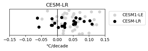
              %%time
              # (Black dots): box-mean trend per CESM-LR member.
              lr_box_series = {m: box_mean_latlon(lr_members[m], weights=lr_area) for m in CESM_LR_MEMBERS}
              lr_box_trend_da = xr.concat(
                  [linear_trend_per_decade(s) for s in lr_box_series.values()], dim="member"
              ).assign_coords(member=CESM_LR_MEMBERS)
              lr_box_trend_da = lr_box_trend_da.compute()
              lr_box_trends = dict(zip(lr_box_trend_da["member"].values, lr_box_trend_da.values))
              lr_box_trends
              
              CPU times: user 1.52 s, sys: 220 ms, total: 1.74 s
              Wall time: 6.46 s
              
              {np.int64(2): np.float64(0.08424489938326829),
               np.int64(3): np.float64(0.051188712409728235),
               np.int64(4): np.float64(0.052287668946329025),
               np.int64(5): np.float64(0.10916964929092499),
               np.int64(6): np.float64(0.02432273740514713),
               np.int64(7): np.float64(0.013541497017552502),
               np.int64(8): np.float64(-0.018232994731698347),
               np.int64(9): np.float64(0.10212831620781637),
               np.int64(10): np.float64(-0.057947584846869474),
               np.int64(11): np.float64(-0.06233954809856511),
               np.int64(12): np.float64(0.07097590385574432),
               np.int64(13): np.float64(-0.016188330807185753),
               np.int64(14): np.float64(0.05856882979162647),
               np.int64(15): np.float64(0.023707360322640307),
               np.int64(16): np.float64(0.0564252525249498),
               np.int64(17): np.float64(0.014323634143355976),
               np.int64(18): np.float64(0.057982488875418896),
               np.int64(19): np.float64(-0.01690756581668129),
               np.int64(20): np.float64(0.022756750923071778),
               np.int64(21): np.float64(0.003083017107088716),
               np.int64(22): np.float64(-0.008576149909311298)}
              
              %%time
              # Ensemble-mean spatial trend map. Only 1° x 21 members x 516 months —
              # far cheaper than the CESM-HR native-grid equivalent.
              lr_member_trend_maps = [linear_trend_per_decade(lr_members[m]) for m in CESM_LR_MEMBERS]
              lr_ensemble_mean_trend = xr.concat(lr_member_trend_maps, dim="member").mean(dim="member").compute()
              
              im = plot_trend_map_latlon(lr_ensemble_mean_trend, "CESM-LR ensemble-mean SST trend 1980-2022")
              plt.colorbar(im, orientation="horizontal", pad=0.05, label="°C/decade")
              plt.show()
              
              ../../../_images/cd8a21ba6d99c8f2f8816a9ae3d66249ce69b85de50f7b6f9fd8817db8a74978.png
              CPU times: user 6.31 s, sys: 378 ms, total: 6.69 s
              Wall time: 10.3 s
              

              CESM1-LE: full ensemble#

              Native gx1v6 POP grid (curvilinear TLAT/TLONG, static — no spurious time dimension on the coordinates the way the CESM-HR product briefly had for member 002). Only a box-mean trend is needed here (no spatial map), so this uses a lightweight curvilinear box-mean directly on TLAT/TLONG/TAREA rather than building a full uxarray Grid for a grid we only ever reduce to one number per member.

              File discovery mirrors the same idea as open_regridded_member in the PRECT notebook: glob, exclude irrelevant variants (here, the OIC sensitivity-run files, which end in 1999 and aren’t part of the main 40-member ensemble), and match historical (20TRC5CNBDRD, 1920-2005) with its RCP8.5 continuation (RCP85C5CNBDRD, 2006-2100) per member. This resolves to the canonical 40-member ensemble (members 001-035, 101-105).

              _CESM1LE_RE = re.compile(r"\.B(20TRC5CNBDRD|RCP85C5CNBDRD)\.f09_g16\.(\d+)\.pop\.h\.SST\.")
              
              
              def discover_cesm1le_members():
                  hist_files, rcp_files = {}, {}
                  for p in CESM1LE_SST_PATH.glob("*.pop.h.SST.*.nc"):
                      if "OIC" in p.name:
                          continue
                      m = _CESM1LE_RE.search(p.name)
                      if not m:
                          continue
                      exp, member = m.groups()
                      (hist_files if exp == "20TRC5CNBDRD" else rcp_files)[member] = p
              
                  return {
                      member: sorted([hp] + ([rcp_files[member]] if member in rcp_files else []))
                      for member, hp in hist_files.items()
                      if member in rcp_files  # need the RCP8.5 continuation to reach 2022
                  }
              
              
              def open_cesm1le_sst_member(files, t0=T_START, t1=T_END):
                  ds = xr.open_mfdataset(
                      files, combine="nested", concat_dim="time",
                      decode_times=xr.coders.CFDatetimeCoder(use_cftime=True),
                      decode_timedelta=False, chunks={"time": 120},
                      data_vars="minimal", coords="minimal", compat="override",
                  )
                  sst = ds["SST"].isel(z_t=0, drop=True).sel(time=slice(t0, t1))
                  return sst, ds["TLAT"], ds["TLONG"], ds["TAREA"]
              
              
              def box_mean_curvilinear(da, tlat, tlon, area):
                  lon = _lon_to_180(tlon)
                  in_box = (lon >= BOX_LON[0]) & (lon <= BOX_LON[1]) & (tlat >= BOX_LAT[0]) & (tlat <= BOX_LAT[1])
                  w = area.where(in_box).where(da.notnull())
                  return (da * w).sum(dim=["nlat", "nlon"], skipna=True) / w.sum(dim=["nlat", "nlon"], skipna=True)
              
              %%time
              cesm1le_files = discover_cesm1le_members()
              print(f"{len(cesm1le_files)} CESM1-LE members:", sorted(cesm1le_files))
              
              40 CESM1-LE members: ['001', '002', '003', '004', '005', '006', '007', '008', '009', '010', '011', '012', '013', '014', '015', '016', '017', '018', '019', '020', '021', '022', '023', '024', '025', '026', '027', '028', '029', '030', '031', '032', '033', '034', '035', '101', '102', '103', '104', '105']
              CPU times: user 4.7 ms, sys: 387 μs, total: 5.09 ms
              Wall time: 15 ms
              
              %%time
              # Opened + reduced to a box-mean series member by member (not batched into one
              # big concat-then-compute like the other sections) — 40 members x static
              # curvilinear coordinates is enough files that building one combined graph
              # isn't necessary for a reduction this cheap, and doing it one at a time keeps
              # any single bad/missing member from failing the whole batch.
              cesm1le_box_trends = {}
              for member, files in cesm1le_files.items():
                  sst, tlat, tlon, tarea = open_cesm1le_sst_member(files)
                  box_series = box_mean_curvilinear(sst, tlat, tlon, tarea)
                  cesm1le_box_trends[member] = float(linear_trend_per_decade(box_series).compute())
              
              cesm1le_box_trends
              
              CPU times: user 9.26 s, sys: 2.16 s, total: 11.4 s
              Wall time: 43.8 s
              
              {'006': -0.04847064288975516,
               '028': 0.004542894239891184,
               '104': 0.1559622498780495,
               '001': 0.07818392356037694,
               '105': 0.05141288976343197,
               '034': 0.07112392812107211,
               '103': 0.11619462365117592,
               '032': -0.0013760487880026173,
               '025': -0.001329948749116515,
               '017': 0.13273525898448799,
               '029': 0.017962198996181185,
               '020': 0.06932654497373628,
               '012': 0.05162017961731694,
               '027': 0.09981950915997934,
               '101': 0.08722229060950347,
               '016': 0.054444365486886845,
               '031': 0.02953002853239713,
               '021': -0.013764537146167745,
               '015': 0.040090892456750155,
               '003': 0.012458878712606878,
               '026': 0.0190190493213518,
               '007': 0.04848457041120325,
               '022': 0.02586521751904811,
               '009': 0.0713587008920485,
               '002': 0.05710319339953996,
               '033': 0.11239166064943532,
               '102': 0.03710833055798484,
               '024': -0.03140953472158226,
               '004': 0.020847123352208775,
               '030': 0.07436095257229544,
               '023': 0.018201466793812335,
               '035': 0.12338432466836471,
               '011': 0.019545622708589252,
               '014': 0.04732996790668888,
               '008': 0.06562990279711503,
               '013': 0.06266348645395234,
               '005': 0.051362463483310555,
               '019': 0.023514678762643598,
               '010': 0.10703517550661651,
               '018': 0.055281486789790925}
              
              rng = np.random.default_rng(0)  # small vertical jitter so overlapping dots stay visible
              
              fig, ax = plt.subplots(figsize=(5, 1.8))
              le_vals = list(cesm1le_box_trends.values())
              ax.scatter(le_vals, rng.uniform(-0.3, 0.3, size=len(le_vals)), color="lightgray", label="CESM1-LE", s=40, zorder=2)
              lr_vals = list(lr_box_trends.values())
              ax.scatter(lr_vals, rng.uniform(-0.15, 0.15, size=len(lr_vals)), color="black", label="CESM-LR", s=40, zorder=3)
              ax.axvline(0, color="black", lw=1)
              ax.set_xlim(-0.15, 0.15)
              ax.set_yticks([])
              ax.set_xlabel("°C/decade")
              ax.legend(loc="upper left", bbox_to_anchor=(1.02, 1.0))
              ax.set_title("CESM-LR")
              plt.tight_layout()
              plt.show()
              
              ../../../_images/29dce783b7226c8dba624bdd66c40daca8ece0c36068522a35fd937da3338646.png
              client.close()
              

              previous

              USCLIVAR’s MESACLIP Atmosphere Whole Ensemble Analysis on Native CESM Mesh with UXarray

              Contents
              • IMPORTS & DASK CONFIG
              • RUN CONFIG (Native Grid - only for CESM-HR)
              • HELPER FUNCTIONS: LINEAR TREND AND BOX MEAN
              • OBSERVATIONS: ERSSTv5, HadISST1, ERA5
              • CESM-HR: NATIVE GRID (uxarray)
              • CESM-LR: REGRIDDED (aave)
              • CESM1-LE: full ensemble

              By UXarray developers and community

              © Copyright UXarray developers.